Deep Learning Take Home Assignment
Converting an 🚀 interview into an offer is a long process. While it may involve various rounds of discussions, we are often given take-home assignments to test our skills on a near real world problem in the preliminary rounds. Although it’s a very good way to judge a candidate’s proficiency in solving a problem, it may be time consuming and sometimes very frustrating when no feedback is given after hours of hard work.
But anyway, in this Deep Learning Interview process, we 🤓 are given a food classification dataset which has 101 classes. Source . We need to analyze and preprocess the dataset as well as build deep learning models for performing food classification. We are free to choose any Deep Learning framework out there. We will use TensorFlow for this excercise.
As this dataset is already present at tensorflow_datasets and can be easily downloaded as a tfds . But, we will download raw data and then preprocess it according to our needs to showcase technical skills as real world data may come in any shape and size.
Judging criteria would be how to format raw data and put in respective directories to be able to fed to model, create train-test split, data visualization, data preprocessing, data augmnetation, input pipelines, modeling (transfer learning, fine tuning), validation, metrics visualization, inference etc.
Bonus: You may get extra points for Deployment
Read this on linkedin
Follow the code here 😀 google colab
connect with me at- blog/github pages , linkedin , twitter , github
Let’s go deeper Food Lovers or should I say Deep Food Lovers 😋
1. Download the data
We download raw data from source and unzip it.
# download raw data
!wget http://data.vision.ee.ethz.ch/cvl/food-101.tar.gz

# unzip the data
!tar xzf food-101.tar.gz #add v for verbose #xvzf
Some data sources are provided with metadata.
# README.txt shows how the directory structure
!cat food-101/README.txt

Structure:
----------
pec/
    images/
        <class_name>/
            <image_id>.jpg
    meta/
        classes.txt
        labels.txt
        test.json
        test.txt
        train.json
        train.txt
2. Create train and test subdirectories
Create train/test subdirectories containing set of images to be fed into model.
def create_train_test(folder):
    """
    creates subfolders for train and test under root dir
    copies files from subfolders(classes) under "/images" to subfolders of "/train" & "/test

    """

    # creates subfolders for train and test under root dir
    for cls in labels:
        os.makedirs(base_dir + folder + '/' + cls)

    # copies image files
    with open (base_dir+"meta/" + folder + ".txt", 'r') as file:
        for f in tqdm(file) :
            shutil.move(src=base_dir+"images/" + f[:-1]+ ".jpg",
                        dst=base_dir+folder+"/" + f[:-1]+ ".jpg" )
3. List number of samples in training and testing folders.
The list is too long…so this piece of code just prints total number of samples.
If we want to list all the files, we can set list_files = True
def list_and_count_files(folder, list_files=False):
    """
    lists number of samples in training and testing folders

    """
    counter = 0
    for root, dirs, files in os.walk(base_dir + folder + "/"):
        for file in files:
            if list_files:
                print(os.path.join(root,file))
        counter += len(files)
    print("[INFO] Total number of samples in {} folder".format(folder), counter)

# avoiding printing the all the file names in the display
# set list_files to true if needed to print file names
list_and_count_files(folder="train",list_files=False)
list_and_count_files(folder="test",list_files=False)
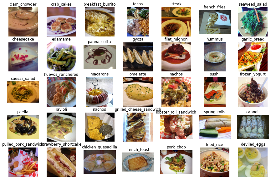
4. Plot sample images from training and testing folders.
This function plots images of random classes from subdirectory.
def display_images(folder):
    """
    plots sample images from training and testing datasets.
    """
    _, axes_list = plt.subplots(5, 7, figsize=(15,10))
    for axes in axes_list:
        for ax in axes:
            ax.axis('off')
            lbl = np.random.choice(os.listdir(base_dir+folder+"/"))
            img = np.random.choice(os.listdir(base_dir+folder+"/" + lbl))
            ax.imshow(PIL.Image.open(base_dir+folder+"/" + lbl+"/"+img))
            ax.set_title(lbl)

# display_images(folder="train")
# display_images(folder="test")
5. Create the train, val, test datasets out of train and test subdirectories
Create train, val and test datasets for model fitting, validation and inference
from tensorflow.keras.preprocessing import image_dataset_from_directory

train_dataset = image_dataset_from_directory(os.path.join(base_dir,"train"),
                                            batch_size=BATCH_SIZE,
                                            image_size=IMG_SIZE,
                                            shuffle=True,
                                            seed=seed,
                                            validation_split=0.2,
                                            subset="training")


val_dataset = image_dataset_from_directory(os.path.join(base_dir,"train"),
                                            batch_size=BATCH_SIZE,
                                            image_size=IMG_SIZE,
                                            shuffle=True,
                                            seed=seed,
                                            validation_split=0.2,
                                            subset="validation")


test_dataset = image_dataset_from_directory(os.path.join(base_dir,"test"),
                                            batch_size=BATCH_SIZE,
                                            image_size=IMG_SIZE,
                                            shuffle=True,
                                            seed=seed)
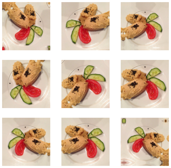
6. Augment the data
Data Augmentation is allowing random manipulations to the input data for training so as to avoid overfitting and giving our model enough variations to generalize well on unseen test data.
Adding a few layers at the start of input pipeline should do the job.
# craete a tensorflow layer for augmentation
data_augmentation = tf.keras.models.Sequential([
                                    tf.keras.layers.RandomFlip('horizontal'),
                                    tf.keras.layers.RandomRotation(0.2),
                                    tf.keras.layers.RandomZoom(0.2)
                                            ])
7. Preview the augmented dataset.
for image, _ in train_dataset.take(1):
    plt.figure(figsize=(10, 10))
    first_image = image[0]
    for i in range(9):
        ax = plt.subplot(3, 3, i + 1)
        augmented_image = data_augmentation(tf.expand_dims(first_image, 0))
        plt.imshow(augmented_image[0] / 255)
        plt.axis('off')
8. Configure dataset for performance
TensorFlow provides great ways to optimize your data pipelines by prefetching data and keeping it ready to be used.
train_dataset = train_dataset.shuffle(500).prefetch(buffer_size=AUTOTUNE)
val_dataset = val_dataset.prefetch(buffer_size=AUTOTUNE)
test_dataset = test_dataset.prefetch(buffer_size=AUTOTUNE)
9. Load pretrained model for transfer learning
We will use InceptionV3 as pretrained model with imagenet weights and without the final layer. For now we will freeze all the layers and train only the final Dense layer.
# Create the base model from the pre-trained model
base_model = tf.keras.applications.inception_v3.InceptionV3(
                                                        include_top=False,
                                                        weights='imagenet',
                                                        input_shape=IMG_SHAPE
                                                            )
print("[INFO] Number of layers in the base model ", len(base_model.layers))

# freeze the base model
base_model.trainable = False
10. Add dense layers on top of pretrained model
Time to compile and run the model.
inputs = tf.keras.layers.Input(shape=IMG_SHAPE)
x = data_augmentation(inputs)
x = tf.keras.applications.inception_v3.preprocess_input(x)
x = base_model(x, training=False) # training=False needed for batchnorm layer
x = tf.keras.layers.GlobalAveragePooling2D()(x)
x = tf.keras.layers.Dropout(0.3)(x)
outputs = tf.keras.layers.Dense(NUM_CLASSES, activation='softmax')(x)

model = tf.keras.models.Model(inputs, outputs)

# compile the model
model.compile(optimizer='adam',
              loss='sparse_categorical_crossentropy',
              metrics=['accuracy'])

# train the model
history = model.fit(train_dataset,
                    batch_size=BATCH_SIZE,
                    epochs=INITIAL_EPOCHS,
                    validation_data=val_dataset)
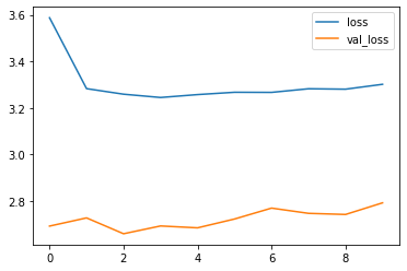
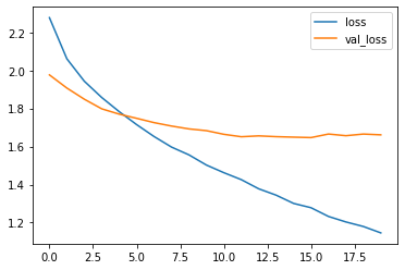
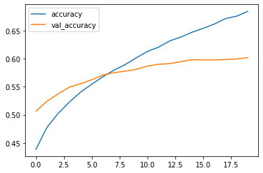
If you see loss/val_loss still improving, you should try to add more epochs to training.
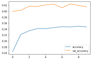
Plot the loss and accuracy curves
history_frame = pd.DataFrame(history.history)
history_frame.loc[:, ['loss', 'val_loss']].plot()
history_frame.loc[:, ['accuracy', 'val_accuracy']].plot()
11. Fine tuning
This step involves opening our model for modifications based on the new data. We would mark few of the top layers as “trainable” and try to train the model with lower learning rate than before so that “pretrained” weights don’t get modified too much. We only want small updates in the pretrained weights.
# un-freeze the model
base_model.trainable = True

# Fine-tune from this layer onwards
fine_tune_at = 250

# Freeze all the layers before the `fine_tune_at` layer
for layer in base_model.layers[:fine_tune_at]:
    layer.trainable =  False

# compile the model. Set very low learning rate.
model.compile(optimizer=tf.keras.optimizers.Adam(learning_rate=1e-5),
             loss='sparse_categorical_crossentropy',
             metrics=['accuracy'])

# train the model with more epochs
history_fine = model.fit(train_dataset,
                        batch_size=BATCH_SIZE,
                        epochs= TOTAL_EPOCHS,
                        validation_data=val_dataset)
Plot the loss and accuracy curves
12. Evaluate on test dataset
loss, accuracy = model.evaluate(test_dataset)
print('Test accuracy :', accuracy)
13. Deploy to gradio
Gradio is the fastest way to demo your machine learning model with a friendly web interface so that anyone can use it, anywhere!
import gradio as gr

def classify_image(inp):
  inp = inp.reshape((-1,) + IMG_SHAPE)
  inp = tf.keras.applications.inception_v3.preprocess_input(inp)
  prediction = model.predict(inp).flatten()
  return {labels[i]: float(prediction[i]) for i in range(101)}

image = gr.inputs.Image(shape=IMG_SIZE)
label = gr.outputs.Label(num_top_classes=3)

gr.Interface(fn=classify_image, inputs=image, outputs=label, interpretation="default").launch(debug=True)
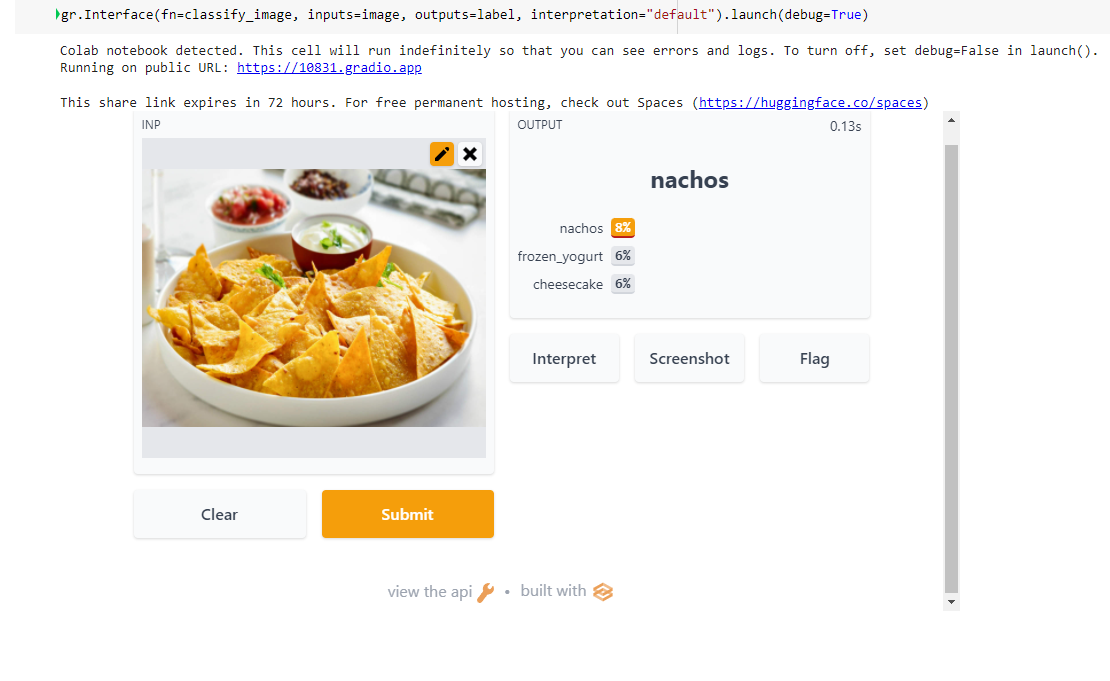
Model was correctly able to predict the food dish was Nachos
14. Conclusion
The reason for low Train/Test accuracy and low confidence score while prediction is because I had to take necessary measures to avoid google colab crashing .
I used all of the Images and classes(101) and therefore had to reduce the image size to 200x200 to avoid crashing of colab. But one can try to reduce the number of classes(subset the data) and train the model again to see very high accuracies ( above 90% accuracy)
I experimented to keep higher batch size also, but had to keep small batch size (32) to avoid colab crashing. One can try to experiment and remeber to tweek the cache/shuffle/prefetch accordingly.
Also I ran the experiment for 10 epochs only. As this is a huge dataset, it would be advised to run for more epochs with larger input shape.
Training from scratch is also a good option as we have good amount of data. But it would need more compute power, that’s why I went ahead with transfer learning, but one can try that also.
Try with different pretrained models.
I ran this using GPU but one can experiment using TPU also.
One can also try to unfreeze whole pretrained model and try to train it with very low learning rate.
Trying different optimizers and callbacks(learning rate schedulers, early stopping etc.) might help improve metrics and run time.
Adding more compute power (colab pro)🤑 would definitely help to prototype/train faster.
Thanks for reading till the end. I hope you learnt something. 🤗
Read other articles on Data Science, Machine Learning, Deep Learning and Computer Vision.